Lion Directional Planes Drawing Model

Introduction to Differential Equations

32 The Logistic Equation

Learning Objectives

Draw the concept of ecology carrying capacity in the logistic model of population growth.
Draw a direction field for a logistic equation and interpret the solution curves.
Solve a logistic equation and interpret the results.

Differential equations can be used to represent the size of a population as it varies over fourth dimension. We saw this in an earlier chapter in the section on exponential growth and disuse, which is the simplest model. A more realistic model includes other factors that affect the growth of the population. In this department, we written report the logistic differential equation and see how information technology applies to the written report of population dynamics in the context of biology.

Population Growth and Carrying Capacity

To model population growth using a differential equation, we kickoff need to introduce some variables and relevant terms. The variable $t.$ volition stand for fourth dimension. The units of time can be hours, days, weeks, months, or fifty-fifty years. Whatsoever given problem must specify the units used in that particular trouble. The variable $P$ will represent population. Since the population varies over time, it is understood to be a part of fourth dimension. Therefore nosotros utilize the notation $P\left(t\right)$ for the population every bit a function of time. If $P\left(t\right)$ is a differentiable function, then the commencement derivative $\frac{dP}{dt}$ represents the instantaneous rate of change of the population as a function of fourth dimension.

In Exponential Growth and Decay, we studied the exponential growth and decay of populations and radioactive substances. An case of an exponential growth part is $P\left(t\right)={P}_{0}{e}^{rt}.$ In this function, $P\left(t\right)$ represents the population at time $t,{P}_{0}$ represents the initial population (population at time $t=0\right),$ and the constant $r>0$ is called the growth rate. (Effigy) shows a graph of $P\left(t\right)=100{e}^{0.03t}.$ Here ${P}_{0}=100$ and $r=0.03.$

An exponential growth model of population.

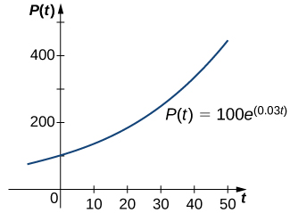
A graph of an exponential function p(t) = 100 e ^ (0.03 t). It is an increasing concave up function starting in quadrant 2, crosses the y axis at (0, 100), and increases in quadrant 1.

Nosotros can verify that the function $P\left(t\right)={P}_{0}{e}^{rt}$ satisfies the initial-value problem

$\frac{dP}{dt}=rP,\phantom{\rule{1em}{0ex}}P\left(0\right)={P}_{0}.$

This differential equation has an interesting estimation. The left-paw side represents the rate at which the population increases (or decreases). The right-hand side is equal to a positive constant multiplied by the current population. Therefore the differential equation states that the rate at which the population increases is proportional to the population at that point in fourth dimension. Furthermore, it states that the constant of proportionality never changes.

One trouble with this function is its prediction that as time goes on, the population grows without spring. This is unrealistic in a real-earth setting. Various factors limit the charge per unit of growth of a particular population, including birth rate, decease rate, nutrient supply, predators, and then on. The growth abiding $r$ normally takes into consideration the nativity and death rates but none of the other factors, and it tin can be interpreted as a net (nascence minus expiry) pct growth charge per unit per unit time. A natural question to ask is whether the population growth rate stays constant, or whether it changes over time. Biologists have found that in many biological systems, the population grows until a sure steady-land population is reached. This possibility is not taken into account with exponential growth. Still, the concept of carrying capacity allows for the possibility that in a given area, merely a certain number of a given organism or animal can thrive without running into resources issues.

Definition

The carrying capacity of an organism in a given surroundings is defined to be the maximum population of that organism that the surroundings can sustain indefinitely.

We use the variable $K$ to denote the carrying capacity. The growth rate is represented by the variable $r.$ Using these variables, nosotros can define the logistic differential equation.

See this website for more than data on the logistic equation.

The logistic equation was first published by Pierre Verhulst in $1845.$ This differential equation can be coupled with the initial condition $P\left(0\right)={P}_{0}$ to form an initial-value problem for $P\left(t\right).$

Suppose that the initial population is pocket-sized relative to the conveying chapters. And then $\frac{P}{K}$ is minor, perhaps close to zero. Thus, the quantity in parentheses on the right-hand side of (Figure) is shut to $1,$ and the right-manus side of this equation is shut to $rP.$ If $r>0,$ so the population grows chop-chop, resembling exponential growth.

However, equally the population grows, the ratio $\frac{P}{K}$ also grows, because $K$ is constant. If the population remains below the carrying capacity, then $\frac{P}{K}$ is less than $1,$ so $1-\frac{P}{K}>0.$ Therefore the right-manus side of (Figure) is withal positive, just the quantity in parentheses gets smaller, and the growth charge per unit decreases as a result. If $P=K$ then the right-paw side is equal to zero, and the population does not alter.

At present suppose that the population starts at a value higher than the carrying capacity. Then $\frac{P}{K}>1,$ and $1-\frac{P}{K}<0.$ Then the right-hand side of (Figure) is negative, and the population decreases. As long as $P>K,$ the population decreases. 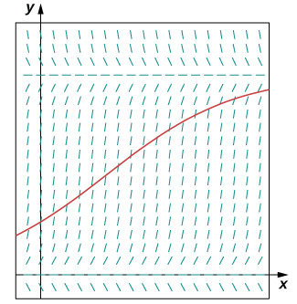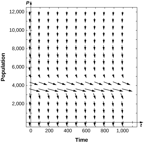It never actually reaches $K$ because $\frac{dP}{dt}$ volition go smaller and smaller, just the population approaches the carrying capacity as $t$ approaches infinity. This assay can be represented visually past way of a phase line. A phase line describes the general behavior of a solution to an autonomous differential equation, depending on the initial status. For the example of a carrying capacity in the logistic equation, the phase line is as shown in (Figure).

A phase line for the differential equation $\frac{dP}{dt}=rP\left(1-\frac{P}{K}\right).$

A diagram of the phase line for the given differential equation. A vertical blue line with arrows on either end has two points marked, at P = K and P = 0, with K > 0. Red arrows point up between 0 and K and down below zero and above K.

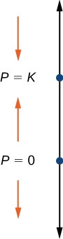
This phase line shows that when $P$ is less than nix or greater than $K,$ the population decreases over time. When $P$ is between $0$ and $K,$ the population increases over time.

Chapter Opener: Examining the Carrying Capacity of a Deer Population

(credit: modification of work by Rachel Kramer, Flickr)

This is a photograph of a deer.

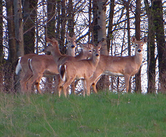
Permit's consider the population of white-tailed deer (Odocoileus virginianus) in the state of Kentucky. The Kentucky Department of Fish and Wild fauna Resources (KDFWR) sets guidelines for hunting and fishing in the state. Before the hunting flavor of $2004,$ it estimated a population of $900,000$ deer. Johnson notes: "A deer population that has plenty to swallow and is not hunted by humans or other predators will double every three years." (George Johnson, "The Problem of Exploding Deer Populations Has No Attractive Solutions," January $12,2001,$ accessed Apr nine, 2015, http://world wide web.txtwriter.com/onscience/Manufactures/deerpops.html.) This observation corresponds to a rate of increase $r=\frac{\text{ln}\left(2\right)}{3}=0.2311,$ so the approximate growth rate is

*** QuickLaTeX cannot compile formula: 23.11\text{%}  *** Error message: File ended while scanning employ of \text@. Emergency cease.

per year. (This assumes that the population grows exponentially, which is reasonable––at least in the curt term––with plentiful food supply and no predators.) The KDFWR also reports deer population densities for $32$ counties in Kentucky, the average of which is approximately $27$ deer per foursquare mile. Suppose this is the deer density for the whole state $\left(39,732$ foursquare miles). The carrying chapters $K$ is $39,732$ square miles times $27$ deer per square mile, or $1,072,764$ deer.

For this awarding, we have ${P}_{0}=900,000,K=1,072,764,$ and $r=0.2311.$ Substitute these values into (Effigy) and class the initial-value problem.
Solve the initial-value problem from part a.
According to this model, what will be the population in $3$ years? Recollect that the doubling time predicted by Johnson for the deer population was $3$ years. How do these values compare?
Suppose the population managed to attain $1,200,000$ deer. What does the logistic equation predict will happen to the population in this scenario?

The initial value problem is
$\frac{dP}{dt}=0.2311P\left(1-\frac{P}{1,072,764}\right),\phantom{\rule{1em}{0ex}}P\left(0\right)=900,000.$
The logistic equation is an democratic differential equation, and then we can utilize the method of separation of variables.
Step 1: Setting the right-mitt side equal to zero gives $P=0$ and $P=1,072,764.$ This means that if the population starts at zero information technology volition never change, and if information technology starts at the carrying capacity, it will never modify.
Step 2: Rewrite the differential equation and multiply both sides by:

$\begin{array}{ccc}\hfill \frac{dP}{dt}& =\hfill & 0.2311P\left(\frac{1,072,764-P}{1,072,764}\right)\hfill \\ \hfill dP& =\hfill & 0.2311P\left(\frac{1,072,764-P}{1,072,764}\right)\phantom{\rule{0.1em}{0ex}}dt.\hfill \end{array}$

Divide both sides by $P\left(1,072,764-P\right)\text{:}$

$\frac{dP}{P\left(1,072,764-P\right)}=\frac{0.2311}{1,072,764}dt.$

Step 3: Integrate both sides of the equation using fractional fraction decomposition:

$\begin{array}{ccc}\hfill \int \frac{dP}{P\left(1,072,764-P\right)}& =\hfill & \int \frac{0.2311}{1,072,764}dt\hfill \\ \hfill \frac{1}{1,072,764}\int \left(\frac{1}{P}+\frac{1}{1,072,764-P}\right)\phantom{\rule{0.1em}{0ex}}dP& =\hfill & \frac{0.2311t}{1,072,764}+C\hfill \\ \hfill \frac{1}{1,072,764}\phantom{\rule{0.1em}{0ex}}\left(\text{ln}|P|-\text{ln}|1,072,764-P|\right)& =\hfill & \frac{0.2311t}{1,072,764}+C.\hfill \end{array}$

Pace 4: Multiply both sides by $1,072,764$ and utilise the quotient rule for logarithms:

$\text{ln}|\frac{P}{1,072,764-P}|=0.2311t+{C}_{1}.$

Here ${C}_{1}=1,072,764C.$ Adjacent exponentiate both sides and eliminate the absolute value:

$\begin{array}{ccc}\hfill {e}^{\text{ln}|\frac{P}{1,072,764-P}|}& =\hfill & {e}^{0.2311t+{C}_{1}}\hfill \\ \hfill |\frac{P}{1,072,764-P}|& =\hfill & {C}_{2}{e}^{0.2311t}\hfill \\ \hfill \frac{P}{1,072,764-P}& =\hfill & {C}_{2}{e}^{0.2311t}.\hfill \end{array}$

Hither ${C}_{2}={e}^{{C}_{1}}$ but after eliminating the absolute value, information technology can exist negative as well. At present solve for:

$\begin{array}{ccc}\hfill P& =\hfill & {C}_{2}{e}^{0.2311t}\left(1,072,764-P\right).\hfill \\ \hfill P& =\hfill & 1,072,764{C}_{2}{e}^{0.2311t}-{C}_{2}P{e}^{0.2311t}\hfill \\ \hfill P+{C}_{2}P{e}^{0.2311t}& =\hfill & 1,072,764{C}_{2}{e}^{0.2311t}\hfill \\ \hfill P\left(1+{C}_{2}{e}^{0.2311t}\right)& =\hfill & 1,072,764{C}_{2}{e}^{0.2311t}\hfill \\ \hfill P\left(t\right)& =\hfill & \frac{1,072,764{C}_{2}{e}^{0.2311t}}{1+{C}_{2}{e}^{0.2311t}}.\hfill \end{array}$

Step 5: To determine the value of ${C}_{2},$ information technology is actually easier to get dorsum a couple of steps to where ${C}_{2}$ was divers. In particular, utilise the equation

$\frac{P}{1,072,764-P}={C}_{2}{e}^{0.2311t}.$

The initial status is $P\left(0\right)=900,000.$ Replace $P$ with $900,000$ and $t$ with zero:

$\begin{array}{ccc}\hfill \frac{P}{1,072,764-P}& =\hfill & {C}_{2}{e}^{0.2311t}\hfill \\ \hfill \frac{900,000}{1,072,764-900,000}& =\hfill & {C}_{2}{e}^{0.2311\left(0\right)}\hfill \\ \hfill \frac{900,000}{172,764}& =\hfill & {C}_{2}\hfill \\ \hfill {C}_{2}& =\hfill & \frac{25,000}{4,799}\approx 5.209.\hfill \end{array}$

Therefore

$\begin{array}{cc}\hfill P\left(t\right)& =\frac{1,072,764\left(\frac{25000}{4799}\right)\phantom{\rule{0.1em}{0ex}}{e}^{0.2311t}}{1+\left(\frac{25000}{4799}\right)\phantom{\rule{0.1em}{0ex}}{e}^{0.2311t}}\hfill \\ & =\frac{1,072,764\left(25000\right){e}^{0.2311t}}{4799+25000{e}^{0.2311t}}.\hfill \end{array}$

Dividing the numerator and denominator by $25,000$ gives

$P\left(t\right)=\frac{1,072,764{e}^{0.2311t}}{0.19196+{e}^{0.2311t}}.$

(Figure) is a graph of this equation.

Logistic bend for the deer population with an initial population of $900,000$ deer.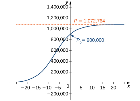
Using this model nosotros can predict the population in $3$ years.

$P\left(3\right)=\frac{1,072,764{e}^{0.2311\left(3\right)}}{0.19196+{e}^{0.2311\left(3\right)}}\approx 978,830\phantom{\rule{0.2em}{0ex}}\text{deer}$

This is far short of twice the initial population of $900,000.$ Remember that the doubling time is based on the assumption that the growth rate never changes, but the logistic model takes this possibility into account.
If the population reached $1,200,000$ deer, then the new initial-value problem would be

$\frac{dP}{dt}=0.2311P\left(1-\frac{P}{1,072,764}\right),\phantom{\rule{1em}{0ex}}P\left(0\right)=1,200,000.$

The general solution to the differential equation would remain the aforementioned.

$P\left(t\right)=\frac{1,072,764{C}_{2}{e}^{0.2311t}}{1+{C}_{2}{e}^{0.2311t}}$

To determine the value of the constant, return to the equation

$\frac{P}{1,072,764-P}={C}_{2}{e}^{0.2311t}.$

Substituting the values $t=0$ and $P=1,200,000,$ you get

$\begin{array}{ccc}\hfill {C}_{2}{e}^{0.2311\left(0\right)}& =\hfill & \frac{1,200,000}{1,072,764-1,200,000}\hfill \\ \hfill {C}_{2}& =\hfill & -\frac{100,000}{10,603}\approx -9.431.\hfill \end{array}$

Therefore

$\begin{array}{cc}\hfill P\left(t\right)& =\frac{1,072,764{C}_{2}{e}^{0.2311t}}{1+{C}_{2}{e}^{0.2311t}}\hfill \\ & =\frac{1,072,764\left(-\frac{100,000}{10,603}\right)\phantom{\rule{0.1em}{0ex}}{e}^{0.2311t}}{1+\left(-\frac{100,000}{10,603}\right)\phantom{\rule{0.1em}{0ex}}{e}^{0.2311t}}\hfill \\ & =-\frac{107,276,400,000{e}^{0.2311t}}{100,000{e}^{0.2311t}-10,603}\hfill \\ & \approx \frac{10,117,551{e}^{0.2311t}}{9.43129{e}^{0.2311t}-1}.\hfill \end{array}$

This equation is graphed in (Figure).

Logistic curve for the deer population with an initial population of $1,200,000$ deer.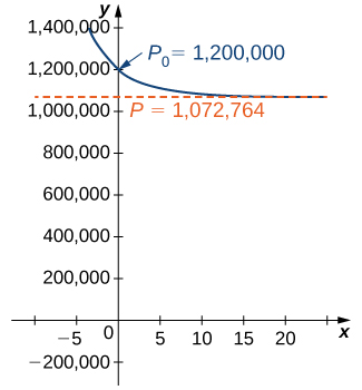

Solving the Logistic Differential Equation

The logistic differential equation is an democratic differential equation, so we tin use separation of variables to find the general solution, every bit nosotros just did in (Figure).

Footstep one: Setting the correct-mitt side equal to zero leads to $P=0$ and $P=K$ as constant solutions. The outset solution indicates that when in that location are no organisms present, the population will never grow. The second solution indicates that when the population starts at the carrying capacity, it will never modify.

Footstep 2: Rewrite the differential equation in the grade

$\frac{dP}{dt}=\frac{rP\left(K-P\right)}{K}.$

Then multiply both sides by $dt$ and divide both sides by $P\left(K-P\right).$ This leads to

$\frac{dP}{P\left(K-P\right)}=\frac{r}{K}dt.$

Multiply both sides of the equation by $K$ and integrate:

$\int \frac{K}{P\left(K-P\right)}dP=\int rdt.$

The left-hand side of this equation can be integrated using partial fraction decomposition. Nosotros exit information technology to you to verify that

$\frac{K}{P\left(K-P\right)}=\frac{1}{P}+\frac{1}{K-P}.$

Then the equation becomes

$\begin{array}{ccc}\hfill \int \frac{1}{P}+\frac{1}{K-P}dP& =\hfill & \int rdt\hfill \\ \hfill \text{ln}|P|-\text{ln}|K-P|& =\hfill & rt+C\hfill \\ \hfill \text{ln}|\frac{P}{K-P}|& =\hfill & rt+C.\hfill \end{array}$

Now exponentiate both sides of the equation to eliminate the natural logarithm:

$\begin{array}{ccc}\hfill {e}^{\text{ln}|\frac{P}{K-P}|}& =\hfill & {e}^{rt+C}\hfill \\ \hfill |\frac{P}{K-P}|& =\hfill & {e}^{C}{e}^{rt}.\hfill \end{array}$

We define ${C}_{1}={e}^{c}$ and so that the equation becomes

$\frac{P}{K-P}={C}_{1}{e}^{rt}.$

To solve this equation for $P\left(t\right),$ first multiply both sides past $K-P$ and collect the terms containing $P$ on the left-mitt side of the equation:

$\begin{array}{ccc}\hfill P& =\hfill & {C}_{1}{e}^{rt}\left(K-P\right)\hfill \\ \hfill P& =\hfill & {C}_{1}K{e}^{rt}-{C}_{1}P{e}^{rt}\hfill \\ \hfill P+{C}_{1}P{e}^{rt}& =\hfill & {C}_{1}K{e}^{rt}.\hfill \end{array}$

Next, factor $P$ from the left-hand side and split up both sides by the other gene:

$\begin{array}{ccc}\hfill P\left(1+{C}_{1}{e}^{rt}\right)& =\hfill & {C}_{1}K{e}^{rt}\hfill \\ \hfill P\left(t\right)& =\hfill & \frac{{C}_{1}K{e}^{rt}}{1+{C}_{1}{e}^{rt}}.\hfill \end{array}$

The last step is to determine the value of ${C}_{1}.$ The easiest way to do this is to substitute $t=0$ and ${P}_{0}$ in identify of $P$ in (Figure) and solve for ${C}_{1}\text{:}$

$\begin{array}{ccc}\hfill \frac{P}{K-P}& =\hfill & {C}_{1}{e}^{rt}\hfill \\ \hfill \frac{{P}_{0}}{K-{P}_{0}}& =\hfill & {C}_{1}{e}^{r\left(0\right)}\hfill \\ \hfill {C}_{1}& =\hfill & \frac{{P}_{0}}{K-{P}_{0}}.\hfill \end{array}$

Finally, substitute the expression for ${C}_{1}$ into (Figure):

$P\left(t\right)=\frac{{C}_{1}K{e}^{rt}}{1+{C}_{1}{e}^{rt}}=\frac{\frac{{P}_{0}}{K-{P}_{0}}K{e}^{rt}}{1+\frac{{P}_{0}}{K-{P}_{0}}{e}^{rt}}$

Now multiply the numerator and denominator of the correct-hand side by $\left(K-{P}_{0}\right)$ and simplify:

$\begin{array}{cc}\hfill P\left(t\right)& =\frac{\frac{{P}_{0}}{K-{P}_{0}}K{e}^{rt}}{1+\frac{{P}_{0}}{K-{P}_{0}}{e}^{rt}}\hfill \\ & =\frac{\frac{{P}_{0}}{K-{P}_{0}}K{e}^{rt}}{1+\frac{{P}_{0}}{K-{P}_{0}}{e}^{rt}}·\frac{K-{P}_{0}}{K-{P}_{0}}\hfill \\ & =\frac{{P}_{0}K{e}^{rt}}{\left(K-{P}_{0}\right)+{P}_{0}{e}^{rt}}.\hfill \end{array}$

We state this event equally a theorem.

Solution of the Logistic Differential Equation

Consider the logistic differential equation subject to an initial population of ${P}_{0}$ with carrying capacity $K$ and growth rate $r.$ The solution to the corresponding initial-value trouble is given past

$P\left(t\right)=\frac{{P}_{0}K{e}^{rt}}{\left(K-{P}_{0}\right)+{P}_{0}{e}^{rt}}.$

Now that nosotros have the solution to the initial-value problem, we can choose values for ${P}_{0},r,$ and $K$ and study the solution curve. For example, in (Effigy) we used the values $r=0.2311,K=1,072,764,$ and an initial population of $900,000$ deer. This leads to the solution

$\begin{array}{cc}\hfill P\left(t\right)& =\frac{{P}_{0}K{e}^{rt}}{\left(K-{P}_{0}\right)+{P}_{0}{e}^{rt}}\hfill \\ & =\frac{900,000\left(1,072,764\right){e}^{0.2311t}}{\left(1,072,764-900,000\right)+900,000{e}^{0.2311t}}\hfill \\ & =\frac{900,000\left(1,072,764\right){e}^{0.2311t}}{172,764+900,000{e}^{0.2311t}}.\hfill \end{array}$

Dividing tiptop and bottom past $900,000$ gives

$P\left(t\right)=\frac{1,072,764{e}^{0.2311t}}{0.19196+{e}^{0.2311t}}.$

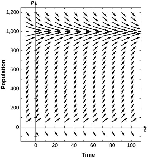
This is the aforementioned every bit the original solution. The graph of this solution is shown once again in blue in (Figure), superimposed over the graph of the exponential growth model with initial population $900,000$ and growth rate $0.2311$ (appearing in greenish). The ruddy dashed line represents the carrying chapters, and is a horizontal asymptote for the solution to the logistic equation.

A comparison of exponential versus logistic growth for the same initial population of $900,000$ organisms and growth charge per unit of

*** QuickLaTeX cannot compile formula: 23.eleven\text{%}.  *** Error message: File ended while scanning use of \text@. Emergency terminate.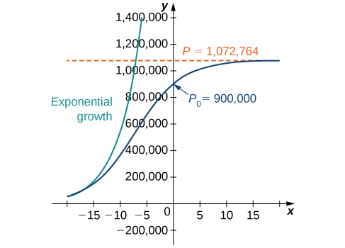

Working under the assumption that the population grows according to the logistic differential equation, this graph predicts that approximately $20$ years earlier $\left(1984\right),$ the growth of the population was very close to exponential. The net growth charge per unit at that time would accept been around

*** QuickLaTeX cannot compile formula: 23.1\text{%}  *** Error bulletin: File ended while scanning utilize of \text@. Emergency stop.

per year. Equally fourth dimension goes on, the two graphs separate. This happens because the population increases, and the logistic differential equation states that the growth rate decreases as the population increases. At the time the population was measured $\left(2004\right),$ it was close to carrying chapters, and the population was starting to level off.

The solution to the logistic differential equation has a point of inflection. To find this betoken, ready the 2nd derivative equal to zero:

$\begin{array}{ccc}\hfill P\left(t\right)& =\hfill & \frac{{P}_{0}K{e}^{rt}}{\left(K-{P}_{0}\right)+{P}_{0}{e}^{rt}}\hfill \\ \hfill {P}^{\prime }\left(t\right)& =\hfill & \frac{r{P}_{0}K\left(K-{P}_{0}\right){e}^{rt}}{{\left(\left(K-{P}_{0}\right)+{P}_{0}{e}^{rt}\right)}^{2}}\hfill \\ \hfill P\text{″}\left(t\right)& =\hfill & \frac{{r}^{2}{P}_{0}K{\left(K-{P}_{0}\right)}^{2}{e}^{rt}-{r}^{2}{P}_{0}{}^{2}K\left(K-{P}_{0}\right){e}^{2rt}}{{\left(\left(K-{P}_{0}\right)+{P}_{0}{e}^{rt}\right)}^{3}}\hfill \\ & =\hfill & \frac{{r}^{2}{P}_{0}K\left(K-{P}_{0}\right){e}^{rt}\left(\left(K-{P}_{0}\right)-{P}_{0}{e}^{rt}\right)}{{\left(\left(K-{P}_{0}\right)+{P}_{0}{e}^{rt}\right)}^{3}}.\hfill \end{array}$

Setting the numerator equal to cipher,

${r}^{2}{P}_{0}K\left(K-{P}_{0}\right){e}^{rt}\left(\left(K-{P}_{0}\right)-{P}_{0}{e}^{rt}\right)=0.$

As long as ${P}_{0}\ne K,$ the unabridged quantity before and including ${e}^{rt}$ is nonzero, so we tin can divide information technology out:

$\left(K-{P}_{0}\right)-{P}_{0}{e}^{rt}=0.$

Solving for $t,$

$\begin{array}{ccc}\hfill {P}_{0}{e}^{rt}& =\hfill & K-{P}_{0}\hfill \\ \hfill {e}^{rt}& =\hfill & \frac{K-{P}_{0}}{{P}_{0}}\hfill \\ \hfill \text{ln}\phantom{\rule{0.1em}{0ex}}{e}^{rt}& =\hfill & \text{ln}\phantom{\rule{0.2em}{0ex}}\frac{K-{P}_{0}}{{P}_{0}}\hfill \\ \hfill rt& =\hfill & \text{ln}\phantom{\rule{0.2em}{0ex}}\frac{K-{P}_{0}}{{P}_{0}}\hfill \\ \hfill t& =\hfill & \frac{1}{r}\phantom{\rule{0.1em}{0ex}}\text{ln}\phantom{\rule{0.2em}{0ex}}\frac{K-{P}_{0}}{{P}_{0}}.\hfill \end{array}$

Observe that if ${P}_{0}>K,$ then this quantity is undefined, and the graph does not have a point of inflection. In the logistic graph, the point of inflection can be seen every bit the betoken where the graph changes from concave up to concave down. This is where the "leveling off" starts to occur, because the net growth rate becomes slower as the population starts to approach the conveying capacity.

$\frac{dP}{dt}=0.04\left(1-\frac{P}{750}\right),\phantom{\rule{1em}{0ex}}P\left(0\right)=200$
$P\left(t\right)=\frac{3000{e}^{.04t}}{11+4{e}^{.04t}}$
After $12$ months, the population will exist $P\left(12\right)\approx 278$ rabbits.

Hint

Beginning determine the values of $r,\phantom{\rule{1em}{0ex}}K,$ and ${P}_{0}.$ And then create the initial-value problem, draw the direction field, and solve the trouble.

Pupil Project: Logistic Equation with a Threshold Population

An improvement to the logistic model includes a threshold population. The threshold population is defined to be the minimum population that is necessary for the species to survive. Nosotros use the variable $T$ to stand for the threshold population. A differential equation that incorporates both the threshold population $T$ and carrying chapters $K$ is

$\frac{dP}{dt}=\text{−}rP\left(1-\frac{P}{K}\right)\left(1-\frac{P}{T}\right)$

where $r$ represents the growth rate, as earlier.

The threshold population is useful to biologists and can be utilized to determine whether a given species should exist placed on the endangered list. A group of Australian researchers say they have adamant the threshold population for whatever species to survive: adults. (Catherine Clabby, "A Magic Number," American Scientist 98(1): 24, doi:10.1511/2010.82.24. accessed Apr nine, 2015, http://www.americanscientist.org/issues/pub/a-magic-number). Therefore we utilize as the threshold population in this projection. Suppose that the environmental carrying capacity in Montana for elk is Set up (Effigy) using the carrying capacity of and threshold population of Assume an annual cyberspace growth rate of
```
*** QuickLaTeX cannot compile formula: 18\text{%}.  *** Mistake message: File ended while scanning use of \text@. Emergency stop.                  
```
Draw the management field for the differential equation from step $1,$ along with several solutions for unlike initial populations. What are the constant solutions of the differential equation? What do these solutions correspond to in the original population model (i.e., in a biological context)?
What is the limiting population for each initial population you chose in step $2?$ (Hint: use the slope field to encounter what happens for various initial populations, i.east., look for the horizontal asymptotes of your solutions.)
This equation can be solved using the method of separation of variables. Even so, it is very difficult to get the solution every bit an explicit function of $t.$ Using an initial population of $18,000$ elk, solve the initial-value problem and express the solution as an implicit function of $t,$ or solve the general initial-value problem, finding a solution in terms of $r,K,T,\text{and}\phantom{\rule{0.2em}{0ex}}{P}_{0}.$

Key Concepts

When studying population functions, different assumptions—such equally exponential growth, logistic growth, or threshold population—lead to different rates of growth.
The logistic differential equation incorporates the concept of a carrying capacity. This value is a limiting value on the population for whatsoever given environment.
The logistic differential equation can be solved for whatever positive growth charge per unit, initial population, and conveying capacity.

Central Equations

For the post-obit problems, consider the logistic equation in the form $P\prime =CP-{P}^{2}.$ Depict the directional field and notice the stability of the equilibria.

$C=3$

$C=-3$

Solve the logistic equation for $C=10$ and an initial condition of $P\left(0\right)=2.$

$P=\frac{10{e}^{10x}}{{e}^{10x}+4}$

Solve the logistic equation for $C=-10$ and an initial status of $P\left(0\right)=2.$

A population of deer within a park has a conveying chapters of $200$ and a growth rate of

*** QuickLaTeX cannot compile formula: 2\text{%}.  *** Error bulletin: File ended while scanning use of \text@. Emergency stop.

If the initial population is $50$ deer, what is the population of deer at any given fourth dimension?

$P\left(t\right)=\frac{10000{e}^{0.02t}}{150+50{e}^{0.02t}}$

The following problems consider the logistic equation with an added term for depletion, either through death or emigration.

[T] The population of trout in a pond is given by $P\prime =0.4P\left(1-\frac{P}{10000}\right)-400,$ where $400$ trout are caught per year. Use your computer or estimator software to draw a directional field and describe a few sample solutions. What practise you expect for the behavior?

A management field with arrows downward for P < one,000, pointing upwards for one,000 < P < 8,500, and pointing down for P > 8,500. Right above P = 8,500, the arrows point down and to the right.

In the preceding problem, what are the stabilities of the equilibria $0<{P}_{1}<{P}_{2}?$

[T] For the preceding trouble, use software to generate a directional field for the value $f=400.$ What are the stabilities of the equilibria?

A direction field with arrows pointing down and to the right. Around y = 4,000, the arrows are more horizontal. The further the arrows are from this line, the more vertical the arrows become.

${P}_{1}$ semi-stable

[T] For the preceding problems, use software to generate a directional field for the value $f=600.$ What are the stabilities of the equilibria?

[T] For the preceding problems, consider the instance where a certain number of fish are added to the pond, or $f=-200.$ What are the nonnegative equilibria and their stabilities?

A direction field with arrows pointing up for P < 10,000 and arrows pointing down for P > 10,000.

${P}_{2}>0$ stable

It is more likely that the amount of fishing is governed by the electric current number of fish present, so instead of a constant number of fish being caught, the rate is proportional to the current number of fish present, with proportionality constant $k,$ equally

$P\prime =0.4P\left(1-\frac{P}{10000}\right)-kP.$

[T] For the previous angling problem, draw a directional field assuming $k=0.1.$ Draw some solutions that exhibit this behavior. What are the equilibria and what are their stabilities?

[T] Use software or a calculator to draw directional fields for $k=0.4.$ What are the nonnegative equilibria and their stabilities?

A direction field with arrows pointing to the right at P = 0. Below 0, the arrows point down and to the right. Above 0, the arrows point down and to the right. The further away from 0, the more vertical the arrows become.

${P}_{1}=0$ is semi-stable

[T] Use software or a calculator to draw directional fields for $k=0.6.$ What are the equilibria and their stabilities?

Solve this equation, assuming a value of $k=0.05$ and an initial condition of $2000$ fish.

$y=\frac{-20}{4\phantom{\rule{0.2em}{0ex}}×\phantom{\rule{0.2em}{0ex}}{10}^{-6}-0.002{e}^{0.01t}}$

Solve this equation, assuming a value of $k=0.05$ and an initial condition of $5000$ fish.

The following problems add in a minimal threshold value for the species to survive, $T,$ which changes the differential equation to $P\prime \left(t\right)=rP\left(1-\frac{P}{K}\right)\left(1-\frac{T}{P}\right).$

Draw the directional field of the threshold logistic equation, assuming $K=10,r=0.1,T=2.$ When does the population survive? When does it go extinct?

A direction field with arrows pointing horizontally to the right forth y = two and y = 10. For P < 2, the arrows betoken down and to the right. For 2 < P < 10, the arrows point up and to the right. For P > 10, the arrows point down and to the right. The further the arrows are from 2 and 10, the steeper they become, and the closer they are from 2 and 10, the more horizontal the arrows become.

For the preceding trouble, solve the logistic threshold equation, assuming the initial status $P\left(0\right)={P}_{0}.$

The following questions consider the Gompertz equation, a modification for logistic growth, which is oft used for modeling cancer growth, specifically the number of tumor cells.

The Gompertz equation is given past $P\left(t\right)\prime =\alpha \phantom{\rule{0.1em}{0ex}}\text{ln}\phantom{\rule{0.1em}{0ex}}\left(\frac{K}{P\left(t\right)}\right)P\left(t\right).$ Describe the directional fields for this equation assuming all parameters are positive, and given that $K=1.$

Assume that for a population, $K=1000$ and $\alpha =0.05.$ Draw the directional field associated with this differential equation and draw a few solutions. What is the behavior of the population?

A management field with arrows pointing down and to the correct for P < 0, upwards for 0 < P < 1,000, and down for P > 1,000. The further the arrows are from P = 0 and P = 1,000, the more vertical they become, and the closer they are, the more horizontal they are.

Show that the population grows fastest when information technology reaches half the conveying capacity for the logistic equation $P\prime =rP\left(1-\frac{P}{K}\right).$

When does population increase the fastest in the threshold logistic equation $P\prime \left(t\right)=rP\left(1-\frac{P}{K}\right)\left(1-\frac{T}{P}\right)?$

$\frac{K+T}{2}$

When does population increase the fastest for the Gompertz equation $P\left(t\right)\prime =\alpha \phantom{\rule{0.1em}{0ex}}\text{ln}\phantom{\rule{0.1em}{0ex}}\left(\frac{K}{P\left(t\right)}\right)P\left(t\right)?$

Below is a table of the populations of whooping cranes in the wild from $1940\phantom{\rule{0.2em}{0ex}}\text{to}\phantom{\rule{0.2em}{0ex}}2000.$ The population rebounded from near extinction afterwards conservation efforts began. The post-obit issues consider applying population models to fit the data. Assume a carrying capacity of $10,000$ cranes. Fit the data assuming years since $1940$ (so your initial population at fourth dimension $0$ would be $22$ cranes).

*Source:* https://www.savingcranes.org/images/stories/site_images/conservation/whooping_crane/pdfs/historic_wc_numbers.pdf
Year (years since conservation began)	Whooping Crane Population
$1940\left(0\right)$	$22$
$1950\left(10\right)$	$31$
$1960\left(20\right)$	$36$
$1970\left(30\right)$	$57$
$1980\left(40\right)$	$91$
$1990\left(50\right)$	$159$
$2000\left(60\right)$	$256$